Partitioning in VVC

VVC’s picture structure adopted a concept from its predecessor, HEVC, wherein a picture is divided into a sequence of coding tree units (CTUs). One CTU consists of an N×N block of luma samples together with two corresponding blocks of chroma samples. The maximum permitted VVC block size is 128×128.
- A picture is divided into one or more tile rows and one or more tile columns.
- A tile is a sequence of CTUs that covers the rectangular region of a picture.
- A slice consists of a whole number of complete tiles, or of a whole number of consecutive and complete CTU rows within a tile of a picture.
Slices and Tiles
There are 2 modes of slices
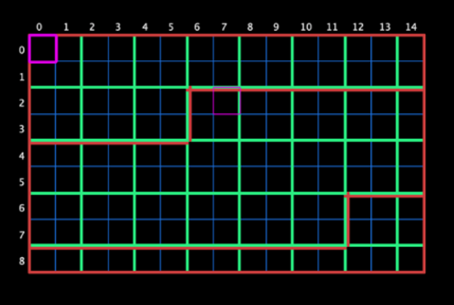
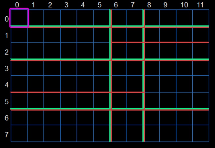
- raster-scan slice: a slice that contains a sequence of complete tiles in a tile raster scan of a picture. Figure 2 shows an example of raster-scan slice partitioning of a picture, where the picture is divided into 40 tiles (8 tile columns × 5 tile rows) and 3 raster-scan slices.
- rectangular slice:
a slice that contains either a number of complete tiles that collectively form a rectangular region of the picture
…or
a number of consecutive complete CTU rows of one tile that collectively form a rectangular region of the picture.
Tiles within a rectangular slice are scanned in tile raster scan order within the rectangular region corresponding to that slice.
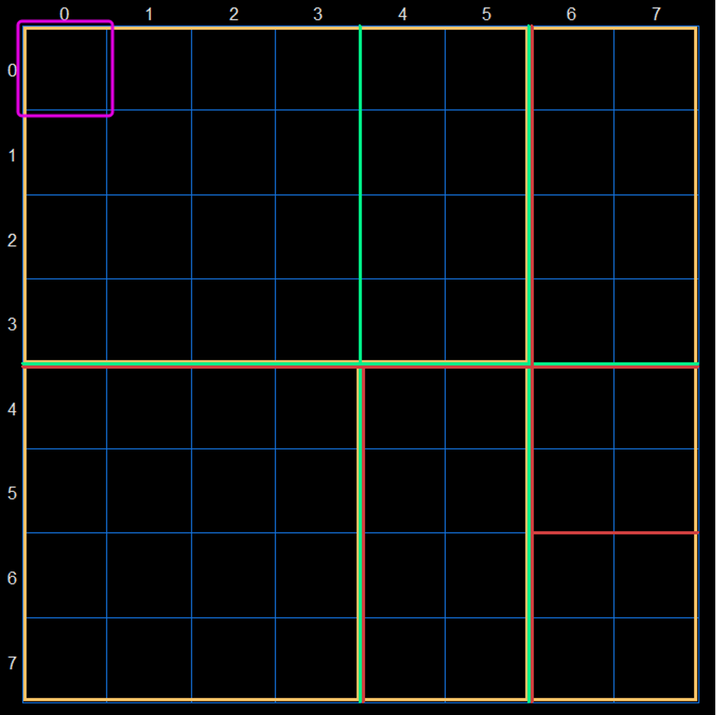
Figure 3 shows an example of rectangular slice partitioning of a picture, where the picture is divided into 40 tiles (8 tile columns × 5 tile rows) and 6 rectangular slices (size in units of tiles 3x3)
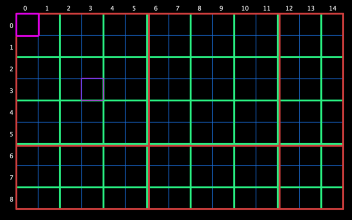
Figure 4 shows an example of rectangular slice partitioning of a picture with several slices in one tile, where the picture is divided into 12 tiles (3 tile columns × 4 tile rows) and 16 rectangular slices.
Subpicture
The main difference between HEVC and VVC in picture partitioning is that the latter is endowed with a new structure called subpicture. Subpicture is developed under the influence of VR, which is currently in vogue. Since the subpictures are completely independent, users could decode only a part of the picture instead of the entire image. Another advantage of subpicture’s independence is that they could be encoded/decoded in parallel. Note that the same applies to slices and tiles as well as they are also independent. They could be encoded/decoded in parallel. A key difference however is that the partitioning of a decoded frame (or a reference frame) into tiles and slices become redundant whereas partitioning of a reference frame into subpictures could bolster the inter prediction process by treating the subpicture boundaries (optionally) as picture boundaries.
Note that subpicture is a rectangular region of one or more slices within a picture. It is crucial to appreciate how the boundaries of tiles, slices and subpictures are related. Each subpicture boundary is also a slice boundary, and every vertical subpicture boundary is always a vertical boundary of some tile.
As we consider dependence of subpictures and tiles, at least one of the following conditions perpetually hold:
- All subpicture’s CTUs belong to the same tile;
- All tile’s CTUs belong to the same subpicture.
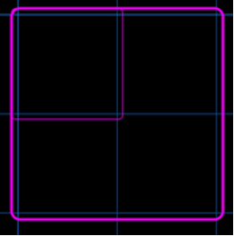
Figure 5 shows an example of rectangular slice partitioning of a picture with several slices in one tile, where the picture is divided into 6 tiles (2 tile columns × 2 tile rows), 6 rectangular slices and 4 subpictures
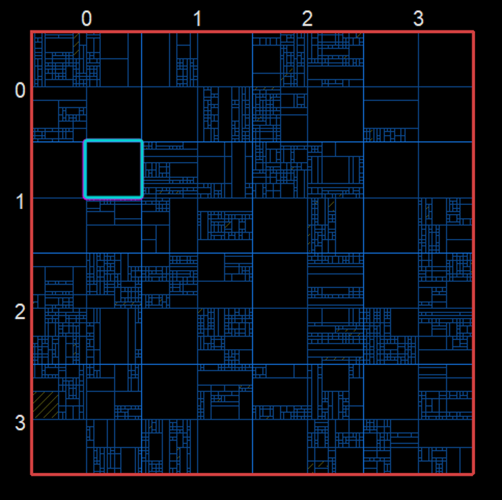
Multi-type Tree structure
Partitioning of the CTUs uses a multi-type tree structure. A quadtree, with nested multi-type tree using binary and ternary splits segmentation structure, replaces the old HEVC concepts of multiple partition unit types*.* That’s to say, it removes the separation of the CU, PU and TU concepts (except as needed for CUs) that are too large for the maximum transform length, and it supports more flexibility for CU partition shapes.
In the coding tree structure, a CU can have either a square or a rectangular shape. A coding tree unit (CTU) is first partitioned by a quaternary tree (a.k.a. quadtree) structure.
Then, the quaternary tree leaf nodes can be further partitioned by a multi-type tree structure. There are four splitting types in the multi-type tree structure,
- vertical binary splitting (SPLIT_BT_VER)
- horizontal binary splitting (SPLIT_BT_HOR)
- vertical ternary splitting (SPLIT_TT_VER)
- horizontal ternary splitting (SPLIT_TT_HOR)
The multi-type tree leaf nodes are called coding units (CUs). This segmentation is used for prediction and transform processing without any further partitioning. This implies that, in most cases, the CU, PU and TU have the same block size in the quadtree with nested multi-type tree coding block structure. The exception is when the maximum supported transform length is smaller than the width or height of the colour component of the CU.
Figure 6 shows a CTU divided into multiple CUs, with a quadtree and nested multi-type tree coding block structure. The quadtree with nested multi-type tree partition provides a content-adaptive coding tree structure comprised of CUs.