Fast skeletonization algorithm


Introduction
Highlighting the skeleton of an object in an image is one of the most popular image processing methods. The skeleton of the image is the data obtained after thinning the objects in the image. In other words, we reduce the number of points belonging to the objects in the image while preserving some of the basic properties of these objects. There are several reasons why this method is interesting today:
- We are reducing the amount of data needed to store an image.
- With a reduced data set, some pattern recognition algorithms work much better.
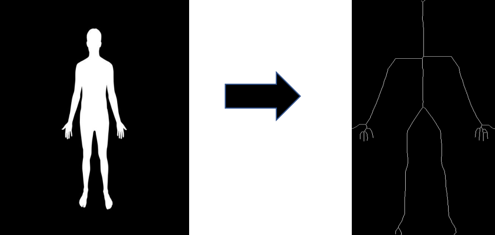
The first mention of such a data compression method dates back to 1959; therefore, this is a relatively old and well-known computer vision problem. However, the question of the efficiency and speed of the algorithm remains open. In this article, we will tell you how to reduce the algorithm's running time by 5-6 times while maintaining the high accuracy of the algorithm. In order to proceed with optimization, we need to describe the skeletonization algorithm itself briefly. An example of the algorithm is shown below.
Definitions
To describe the algorithm, we need to introduce several auxiliary concepts. To simplify the process, we will consider only binary images where all objects are white, and the background is black.
We need a set of eight points, indicated in the table below.
| N3(P) | N2(P) | N1(P) |
| N4(P) | P | N0(P) |
| N5(P) | N6(P) | N7(P) |
Table 1.
The set of N(P) is called the 8–neighbors of P.
"Interior" refers to the points that have all four neighbors in the directions: N0(P), N2(P), N4(P), N6(P).
All points that are not "Interior" but belong to the object (white dots) are called boundary points. C8(P) refers to the number of 8 connected components in N(P).
“Simple” are the points that are boundary and C8(P) = 1.
“Perfect” configuration of points refers to the following configuration: P (perfect point) is a point of the object (white point), N2i(P) is an internal point of the object (also white point), N2i+4(P) is not a point of the object (background).
Problem statement
We need to get the skeleton of the image while preserving the basic topological properties of the object. It is also necessary to optimize the running time of the algorithm. It is important to note that the result of the algorithm should have the following properties:
- The resulting representation of the object should be thin (at least the skeleton should not contain “simple” points).
- The resulting representation of the object should preserve the structural and topological properties of the object. (Basically, the algorithm should not change the number of connected components of the object.)
- It should be possible to reconstruct the image based on the acquired skeleton.
Skeletonization algorithm
So, we have the original binary image, shown below.

The algorithm is divided into three stages: preprocessing, main, and final.
At the preprocessing stage, we need to identify the boundaries of the object. In other words, we form a vector of boundary points that are both “simple” and “perfect”.
We also place the object in a separate image. The background value is set to 0, the value of the boundary points is set to 1, and the value at the points belonging to the interior of the object is set to -1. We also introduce the concept of a fire level as the current value in this particular image, incremented by 1.
At the main stage the skeleton of the object is being formed.
At this stage we are using some modifications of the "prairie-fire algorithm".
Short description:
For each point obtained after the first stage, we look at a 4-connected neighborhood; if the pixel value in the neighborhood is not background and is not equal to the current fire level, then we add this point to the vector of points suspected of being deleted. We also set the pixel value at the point itself as the background value (0). Next, it is necessary to transform the vector of boundary points, which are perfect and simple, from the vector of points suspected of being deleted. We will continue to perform this stage until the vector of suspicious points turns out to be empty.
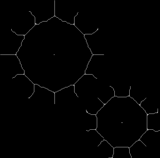
At the third and final stage, we need to make the skeleton single-pixel. Therefore, we remove the remaining “simple” points that do not belong to the skeleton of the object in the image. As a result, we have a thin and continuous skeleton of the object, as shown in Figure 3.
The second stage is the most time-consuming. Note that it is complicated to carry out a successful parallel implementation of algorithms based on the "prairie-fire algorithm" due to the fact that each iteration of the loop of this stage is not independent; the reduction operation will take quite a long time.
So, how can we speed up this algorithm?
Acceleration
We found out that using libraries that run the program in parallel does not give a significant acceleration. We use the scaling and linear interpolation method to speed up the algorithm.
We need to compress the image several times and run the skeleton algorithm described above. The algorithm will work 7-8 times faster by reducing the number of pixels, depending on the compression parameter. It is important to understand that this operation will practically not affect the algorithm's quality.
After receiving a compressed image of the object's skeleton several times, we need to restore its original size.
In this case, we have two ways:
- Scale the resulting image to its original dimensions.
- Transfer the points of the skeleton, multiplying the coordinates by the compression ratio, to an empty (black) image of the desired size.
Let's take a closer look at the first option as the scaling operation is not expensive in terms of computing resources for binary images. Therefore, restoring the skeleton to the desired size in this way will practically not affect the speed, which is a plus. However, by scaling in this way, we will get thickening of the skeleton. The thickening will be proportional to the degree of compression. The thickening contradicts one of the requirements that we imposed on the skeleton in the beginning of this article. (The skeleton must be thin!) Thus, this option of restoring the size does not suit us.
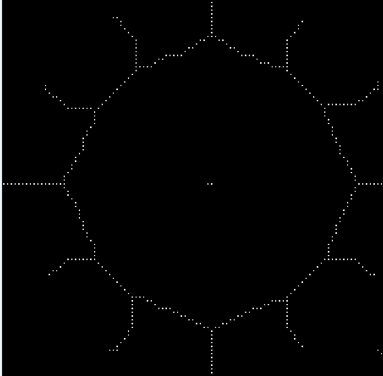
So, we transfer the points by multiplying their coordinates by the compression ratio. Figure 4 shows the part of the object obtained at this stage.
As expected, a gap was formed between each pair of points of the resulting skeleton when using this method. If we leave the skeleton in this form, then we cannot say that it does not change the topological properties of the original object. In addition, there is no guarantee that such a skeleton can still be restored. In this case, interpolation will help us. This approach will not affect the image quality with a fairly small partition. For simplicity, we will use linear interpolation. In general, of course, you can use cubic, linear, quadratic, or any other type of interpolation can be used here. However, it is crucial to understand that achieving a smoother skeleton is more time consuming.
Thus, we must decide how to connect pairs of points. At this stage, there are many ways to connect points, we will consider just a few of them. So, another modification of the "prairie-fire algorithm" will be used to connect the points.
Short description:
We need to look at each pixel of the image. When we reach a white pixel, we add it to the vector, and all the white pixels in the 8-connected neighborhood are added to the stack. Next, we take the pixels out of the stack and perform with them the same procedure. We repeat these steps until the stack is empty.
At the output of this algorithm, we will get a vector of points. Most of the elements of this vector are constructed according to the following rule: each next point is a neighbor of the previous one.
The last step is to connect the neighboring elements of this vector with lines.
Let's look at another way to connect the points:
For each point, we find the nearest point in the sense of Euclidean distance and connect these points. In practice, it has been shown that if we move in one direction vertically and in another direction horizontally, we will be able to minimize the number of gaps. Also, note that each iteration is independent; therefore, it becomes possible to use a parallel loop. Due to parallelism, this method is quite fast.
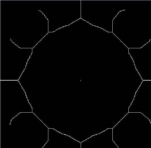
To completely avoid spaces, we apply the bitwise operation "or" to both methods described above. Thus, we have obtained an image skeleton that meets all the requirements defined at the beginning of the article. Figure 5 shows a section of the object after connecting the points.
Conclusion
We have implemented the skeletonization algorithm and obtained a representation of the object in the image that meets the following requirements:
- The skeleton does not contain simple points.
- The skeleton reflects the main structural and topological properties of the object.
- It is possible to restore the original image from the skeleton.
To analyze the result of the algorithm acceleration, we conducted several tests for images with different resolutions. The histogram below shows the execution time (ms) of the algorithm before (in blue) and after (in purple) the optimization.
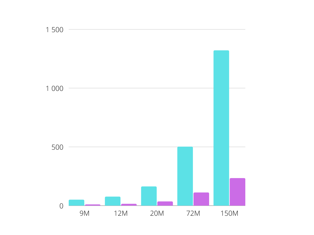
We conclude that using scaling and linear interpolation, we obtained an impressive acceleration of the algorithm for images. In conclusion, it is worth adding that such optimization can be generalized for a certain class of contour search problems on binary images.
References
[1] U. Eckhardt, L. Latecki. (1995). Well–composed sets.
[2] U. Eckhardt, L. Latecki. (1996). Invariant Thinning and Distance Transform. “prairie-fire”