BD-rate: one name - two metrics. AOM vs. the World.

I came up with the idea for this article after conducting a series of experiments while writing another article for AV1-AV2 codec comparison. The main result at the time was to get a stream-averaged BD-rate. This metric was given as a proof of improvements in codec quality. It was at that time that I had to switch from the traditional way of measuring the metric to the one used by AOM, according to their common test conditions (AOM-CTC). But the difference interested me, and I'm here to clarify the situation about this widely used metric.

This article is structured as follows. In the first chapter, I will go through the basic steps of calculating BD-Rate. In the second chapter, I will illustrate the difference in results when calculating the metric with a specific example. In chapter three, I will look at the difference from a mathematical point of view. A conclusion will follow.

Calculating BD-rate

A codec quality comparison experiment consists of a series of encoding, decoding, and metrics calculations on different iterated parameters (bitrate, qp, cq-level, etc.). This way, RD-curves (points on the bitrate-metrics graph) will be built. We use the new version of VQ Probe 2.3.0 for testing given results for the following metrics: PSNR, VMAF, SSIM, CIEDE 2000, CAMBI, MS-SSIM. These metrics help measure the quality of encoded video. Still, more top-level meta-metrics are needed to assess the codec's quality. So, it is common to use BD-Rate.

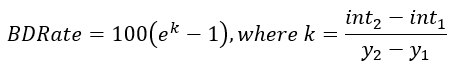
BD-Rate (Bjontegaard delta rate) allows the measurement of the bitrate reduction offered by a codec or codec feature while maintaining the same quality as measured by objective metrics. The BD-Rate method was described in “Calculation of Average PSNR Differences between RD-curves” in 2001 by Bjontegaard [1]. It is a function of two RD curves: a reference curve and a test curve (order is important). BD-Rate is measured as a percentage. BD-rate is 0% when the calculated metrics are the same. When the test shows better results than the reference, the BD-Rate value is less than zero.

If the test is better than the reference, BD-Rate is negative.

Actually, the RD-curve is an approximation; in fact, there is no curve. There is a group of points where each corresponds to one encoded stream. Looking ahead, this is what makes the difference.

Having all the data prepared, the calculation [1] has the following steps.

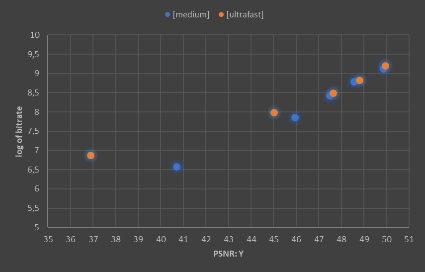
Step 1. Change axes to logarithmic and transpose. Thus, metric-bitrate to log_bitrate-metric.

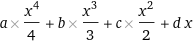
Step 2. Cubic polynomial approximation. This numerical method fits the coefficients of a cubic polynomial by minimizing the standard deviation of the function from the data. Returns four numbers: a, b, c, d.

Step 3. Set integration boundaries. We want to compare RD-curves under the same conditions, but they have different ranges, so we need to trim the data.

The left-hand boundary is defined as the maximum of the minimum values of the two data sets. The right-hand boundary is defined as the minimum of the maximum values of the two data sets.

Step 4. Calculate the area under the curve, i.e., calculate the integral of the function of step 2 within the limits of step 3.

Step 5. Get BD-Rate value.

Experiments

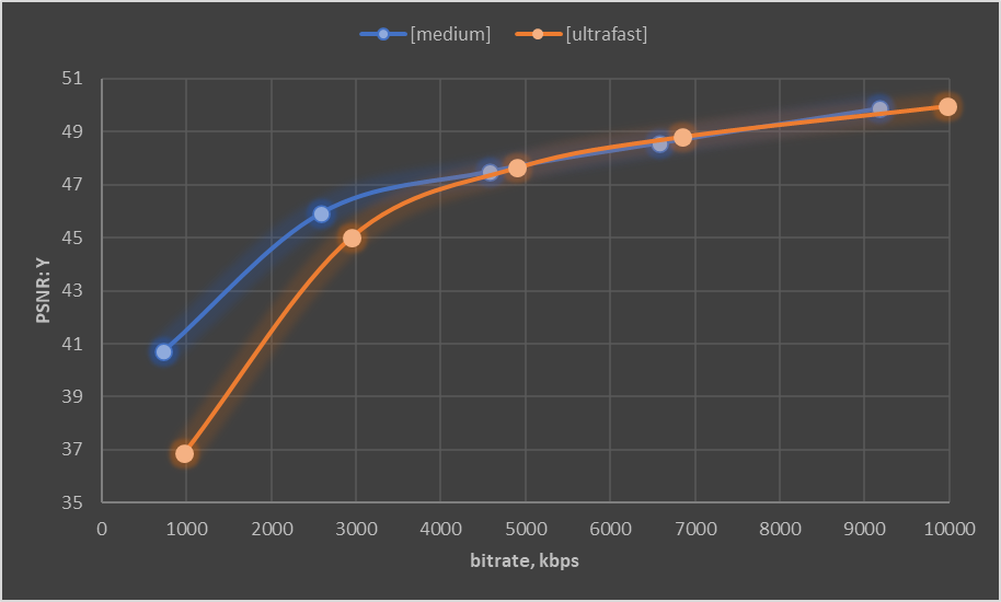
For this series of experiments, I encoded FourPeople_480x270_60.y4m (a5–270p selection from AOM-CTC streams). Encoding was done with libx264 codec on medium and ultrafast presets. Target bitrates are 1000, 3000, 5000, 7000, 10000 kbps. A series of experiments was done with ViCueSoft’s Codec Test Platform (currently under development).

The results of the measurements are shown in the table.

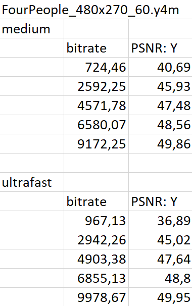
I found the algorithms described in the previous chapter in the implementations: on python (Joao Ascenso, JaymeWX), on excel (Tim Bruylants, ETRO, Vrije Universiteit Brussel). VQProbe runs on C++ implementation. All of these executions are based on approximation by a cubic polynomial (more on this in the next chapter). All these programs returned the same result BD-Rate=52.9%. At the same time, AOM’s BD-Rate gives a result of 41.25%.

Taking a closer look reveals the difference. Using python, the former uses the polyfit function of the numpy library. At the same time, AOM interpolates the RD-curve using pchip_interpolate of the scipy library and thus uses the Piecewise Cubic Hermite Interpolating Polynomial (PCHIP).

Intermediate step data:

Polynomial interpolation gave a=-0.00417, b=0.577055, c=-26.2749, d=400.8928 (equation factors for medium preset step 2 of previous chapter). a=0.001237, b=-0.15458, c=6.551819, d=-86.5756 — for ultrafast.

The integration was made within a boundary between 40.69 and 49.86 (step 3 of the previous chapter).

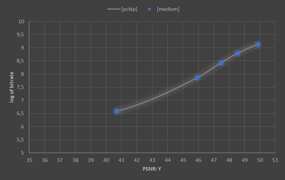
The medium preset calculated area under the graph is 70.57 (for polynomial interpolation) and 71.07 (for PCHIP interpolation). For ultrafast preset: 74.47 and 74.23 correspondingly (step 4 of the previous chapter).

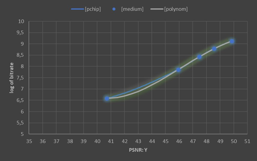
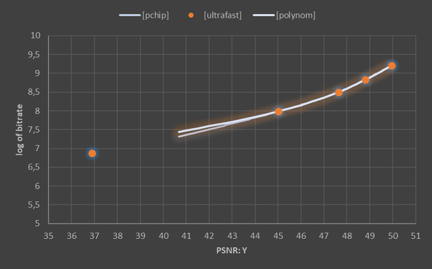
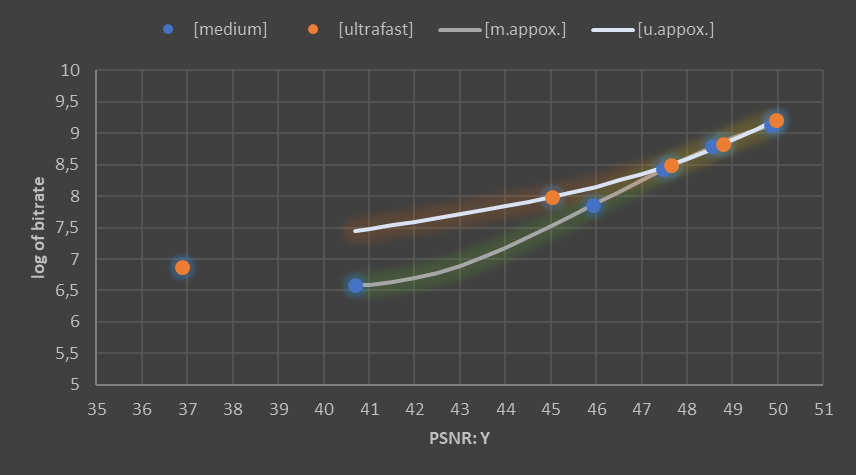
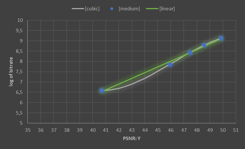
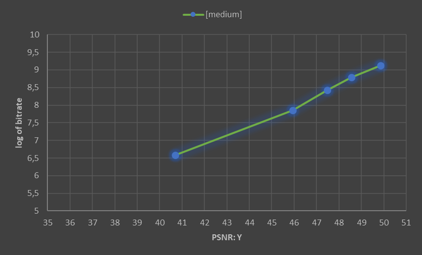
These pictures explain the difference in the results. Different curves mean different areas under the graph and consequently different BD-Rates. So the rarer the dots, the greater the possible divergence in interpolation. For a more detailed look at the mathematical part of interpolation, see the following chapter.

Numerical analysis

In this chapter, I would like to explain how the used python libraries are structured from the mathematical point of view.

Polyfit

Least-squares polynomial fit. That is an approximation by such a polynomial for which the sum of squares of the difference between values of the polynomial and the experiment will be minimum.

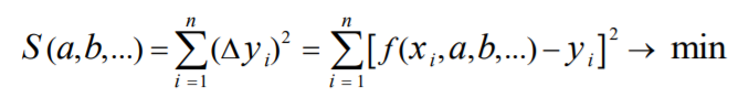
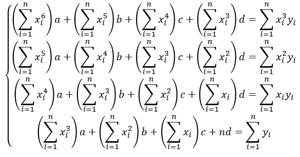
Let’s look at a simple linear least-squares interpolation. According to the necessary criterion of extremum, the partial derivatives of function must be equal to zero. So, the general view turns into this system of equations:

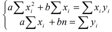
Using the examples of this article, the solution gives the following results:

a=0.28, b=-4.83 for y=ax+b

The same only with a more complex system of equations concerns higher orders of polynomials.

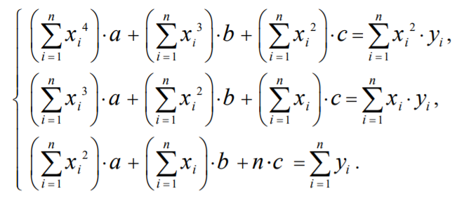
Using the examples of this article, the solution gives the following results:

a=-0.00417, b=0.577055, c=-26.2749, d=400.8928 for cubic polynomial

Python's numpy.polyfit has a third argument (integer) — degree of the fitting polynomial.

np.polyfit(PSNR, lR, 3)

Note the following two things in passing. First, the approximated polynomial does not have to pass through the measurement points, thus assuming the stochastic nature of the measurements. Second, a higher-order polynomial does not mean higher accuracy — high-order polynomials may oscillate wildly.

PCHIP

The Piecewise Cubic Hermite Interpolating Polynomial is a set of splines that goes precisely through the measurement points, whereas the approximated polynomial only minimizes the error. However, this interpolation also assumes different function behavior in different sections.

The simplest case of interpolation with splines (linear) is points connected by lines — finding their equations is not difficult.

For PCHIP, the interpolant uses monotonic cubic splines to find the value of new points x and the derivatives there. Once you have the values and the values of the derivatives at the extreme points, you can start constructing the cubic spline. The Hermite form interpolation theorem proves the possibility and uniqueness of such a construction.

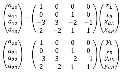
The result, presented in matrix form, will be as follows:

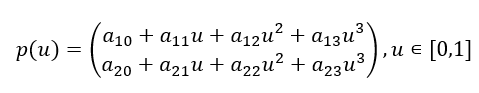
Its arguments can be found from the following ratios:

Python’s scipy.interpolate.pchip_interpolate has the third argument — array of desired interpolated x-values.

scipy.interpolate.pchip_interpolate(qmetrics1, logbr1, samples)

The result looks like this:

Conclusion

In the end, it seems reasonable to draw not the prettiest approximation but the most accurate one in at least some sense. If we assume the logarithmic character of bitrate-PSNR dependence, then linear approximation for log_bitrate-PSNR can also be used. The cubic approximation is the classic one — most people use it. It is worth keeping in mind that any approximation has its inaccuracies, at least because the quality metrics do not quite match the human perception of quality. In any case, the rules should be the same for a metric with the same name.

References

[1] Bjøntegaard, G. (2001). Calculation of Average PSNR Differences between RD-curves.

This article is written by Valery Zimichev, team lead of the test automation department at ViCueSoft company. ViCueSoft specializes in writing software for video analysis and testing codecs. Suppose you are looking for a way to optimize and improve the quality of video transferring or streaming services. In that case, you might want to try our products. Thanks for your attention.