Measuring video quality - a detailed guide

As you might know, we position ourselves as a video quality analysis company. This article demonstrates some aspects of estimating codec quality and how we visualize and evaluate data.
Quality
Do an experiment. Start with the quality test. For example, we should compare some encoder modes. The general steps of such a pipeline will be the next. First of all, we need to encode the entered data; usually, they are raw bitstreams with .yuv extension; then decode the encoded files; the last step is to compare decoded files with the original input streams using some metrics tool. We need some experimental data such as input files - bitstreams and the instructions for internal validation tools. The instructions consist of command blocks for each step of an experiment pipeline. There are the following parts: encoding, decoding, and the measuring metrics tool. Like on the scheme.

Per-frame and RD-curves
Run checking quality pipeline with several bitstreams and some options: encoding, decoding, and metrics tool. These steps are performed within the internal validation framework; more info is presented in the article. Each step of the pipeline is in a separate instruction block. More details are shown below.
- tb::stages:
- label: encoding
instruction: encode() - label: decoding
instruction: decode() - label: metrics
instruction: metrics()
- label: encoding
We iterate over all options that we want to check. We will check codecs in this case. Encode several streams with the same modes. Change only one parameter, which is the codec. They are AVC (h264) and HEVC (h265), for example. Run encoding with bitrate sequence from 1000 to 20000 Mbits. Then run the decoding streams produced on the previous step. There are the same commands for each iteration. The next step is collecting quality metrics from comparing the input stream, which we have used for encoding with the output decoded raw file. Metrics for each frame and the average for all stream frames such as PSNR and MS-SSIM will be used for plotting graphs.
tb::instructions:
- encode:
- label: encoding
- command: encode_tool {:args.codec}
- args:
- name: bitrate
call: '-b {:args.bitrate}' - name: frames
- name: input_stream
call: '-i {}'
value: '{:streams.stream_name}.yuv' - name: encoded_file
call: '-o {}'
value: 'encoded.{:args.bitrate}.{:streams.stream_name}.{:args.codec}'
- name: bitrate
decode:
- label: decoding
- command: decode_tool {:args.codec}
- args:
- name: encoded_file
call: '-i {}'
value: 'encoded.{:args.bitrate}.{:streams.stream_name}.{:args.codec}' - name: decoded_file
call: '-o {}'
value: 'decoded.{:args.bitrate}.{:streams.stream_name}.{:args.codec}.yuv'
- name: encoded_file
metrics:
- label: metrics
- command: metrics_tool
- args:
- name: input_file_1
call: '-i1 {}'
value: '{:streams.stream_name}.yuv' - name: input_file_2
call: '-i2 {}'
value: 'decoded.{:args.bitrate}.{:streams.stream_name}.{:args.codec}.yuv' - name: metrics
call: 'psnr all mssim all'
- name: input_file_1
args:
- codec:
- h265
- h264
- bitrate:
- 1000
- 3000
- 5000
- 7000
- 10000
- 15000
- 20000
streams:
- stream_name: snow_road
- stream_name: sky
- stream_name: sea
- stream_name: seawave
- stream_name: flowers
We have another file with commands for charting per-frame metrics plots and RD-curves. It looks like the next.
RD:
- sheets:
- streams
- metrics:
- avg Y-MSSIM
- avg Y-PSNR
per-frame:
- sheets:
- streams
- metrics:
- Y-PSNR
- Y-MSSIM
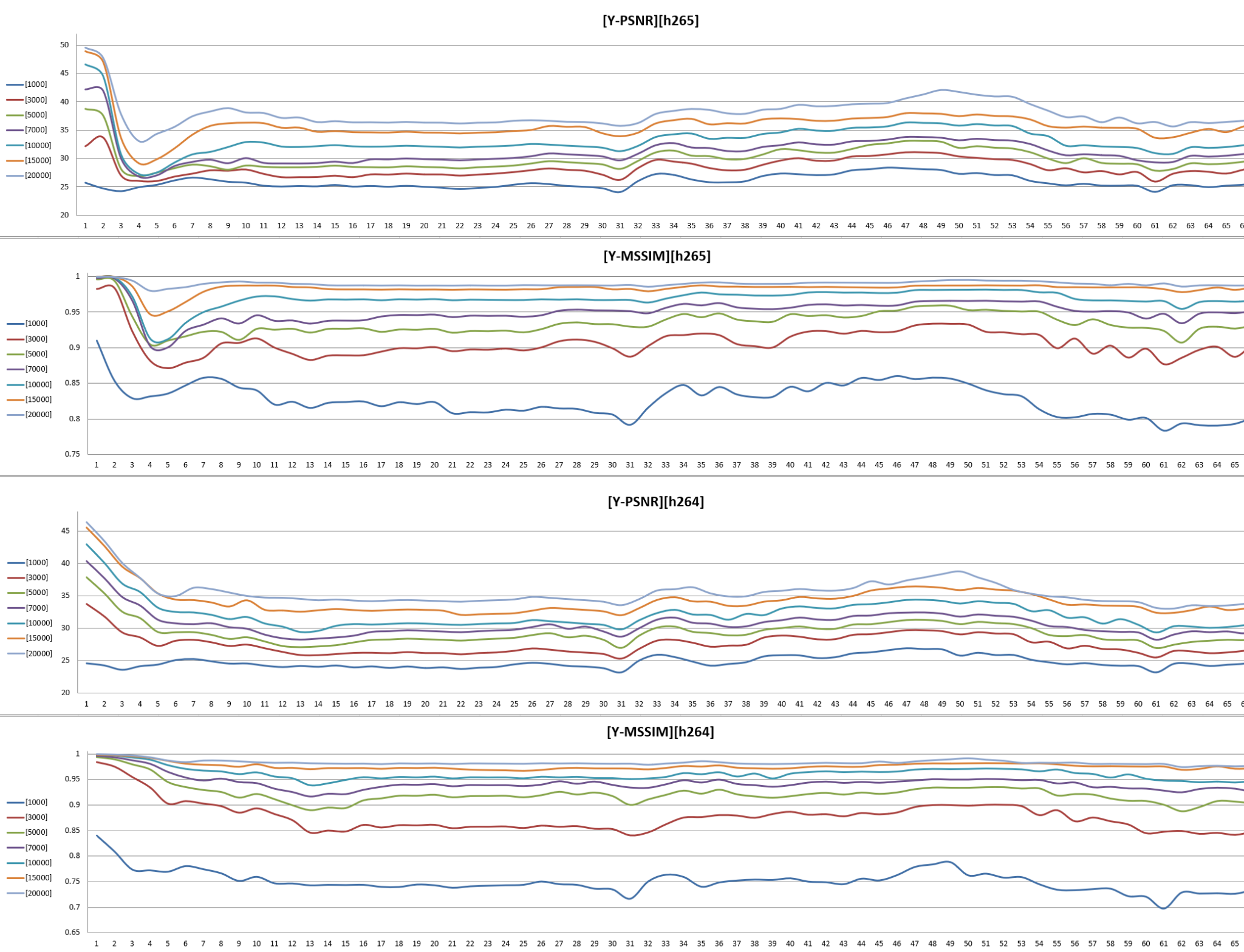
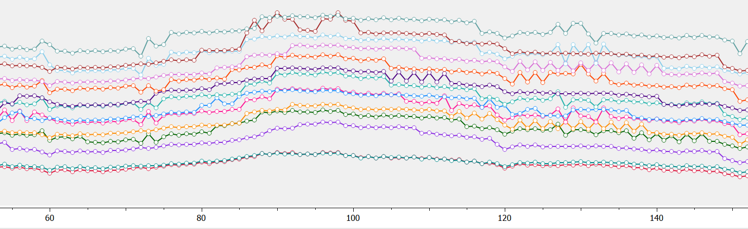
Look at some per-frame plots.
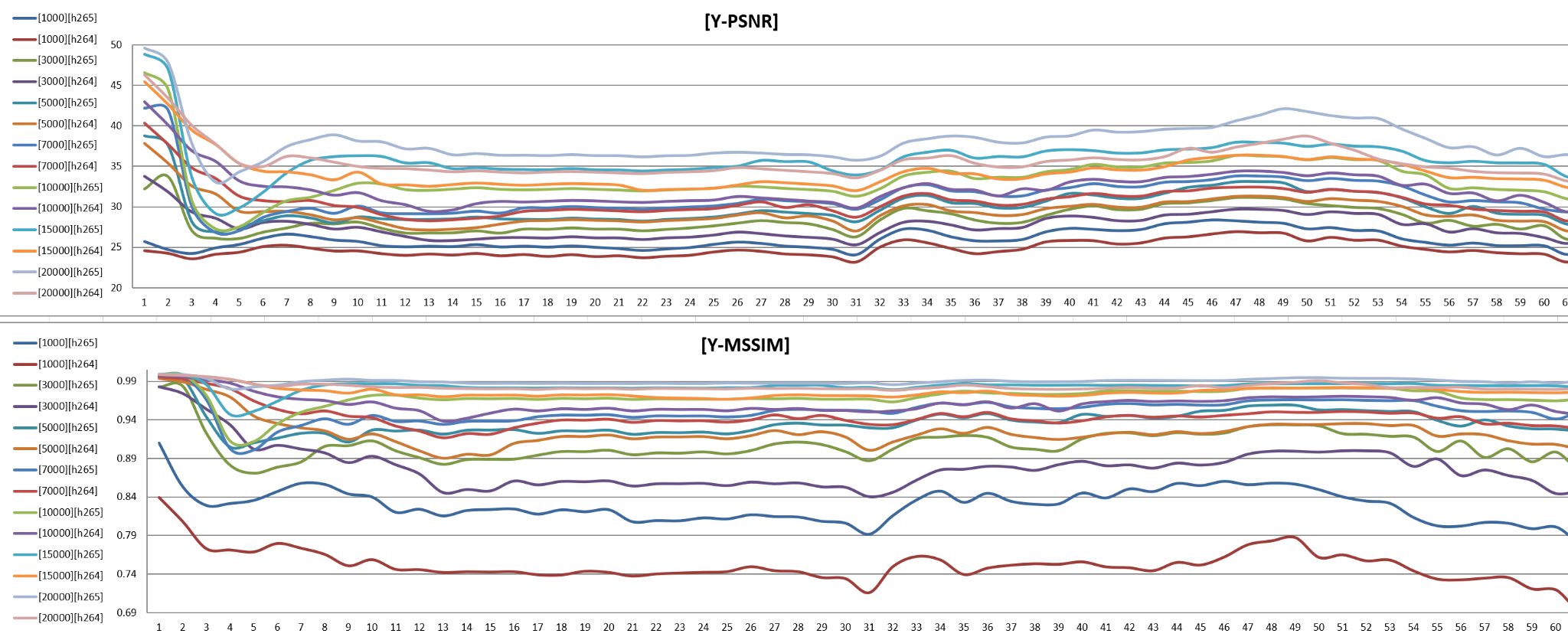
Lines on the plot show quality on each frame. There are shown per-frame PSNR and MS-SSIM metrics in different bitrates and some codecs. Hide some plots for researching quality. We can see that pairs often consist of different codecs, and the same bitrate differs, and one item is of better quality than the other.
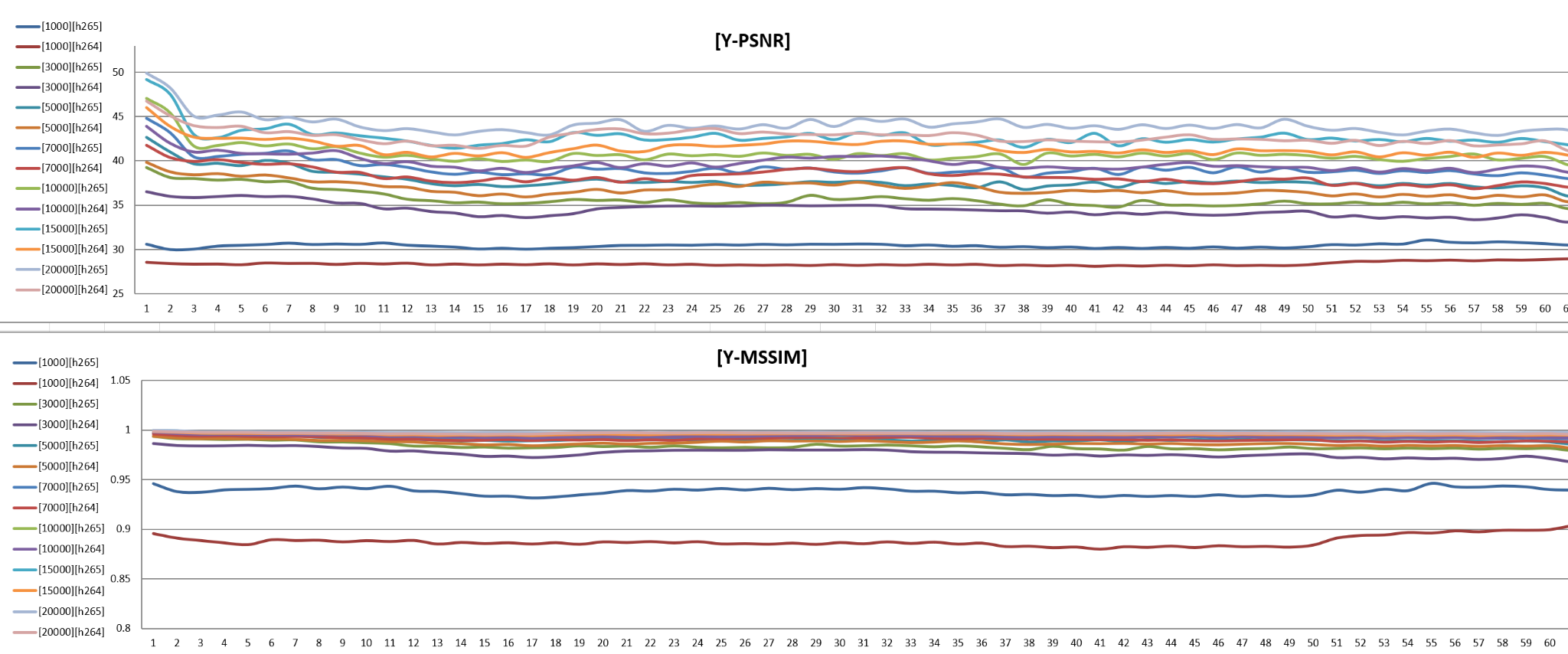
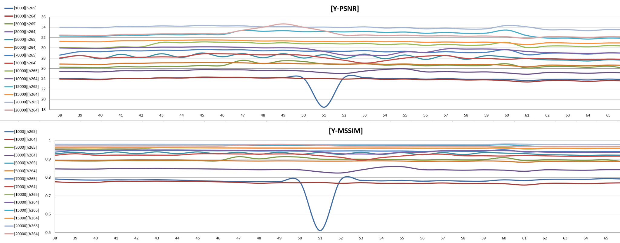
Let's look at a more detailed view - separate plots, make it different for each codec and metric.
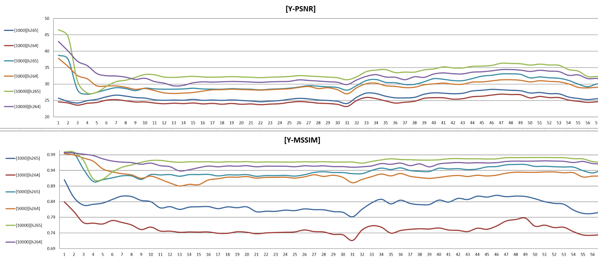
You might have noticed that quality differs between bitrates for the same codec. Lower bitrate means worse quality; higher bitrate means better quality. But sometimes, we can face unusual behavior and find decreased quality on some frames, like in the picture below.
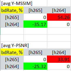
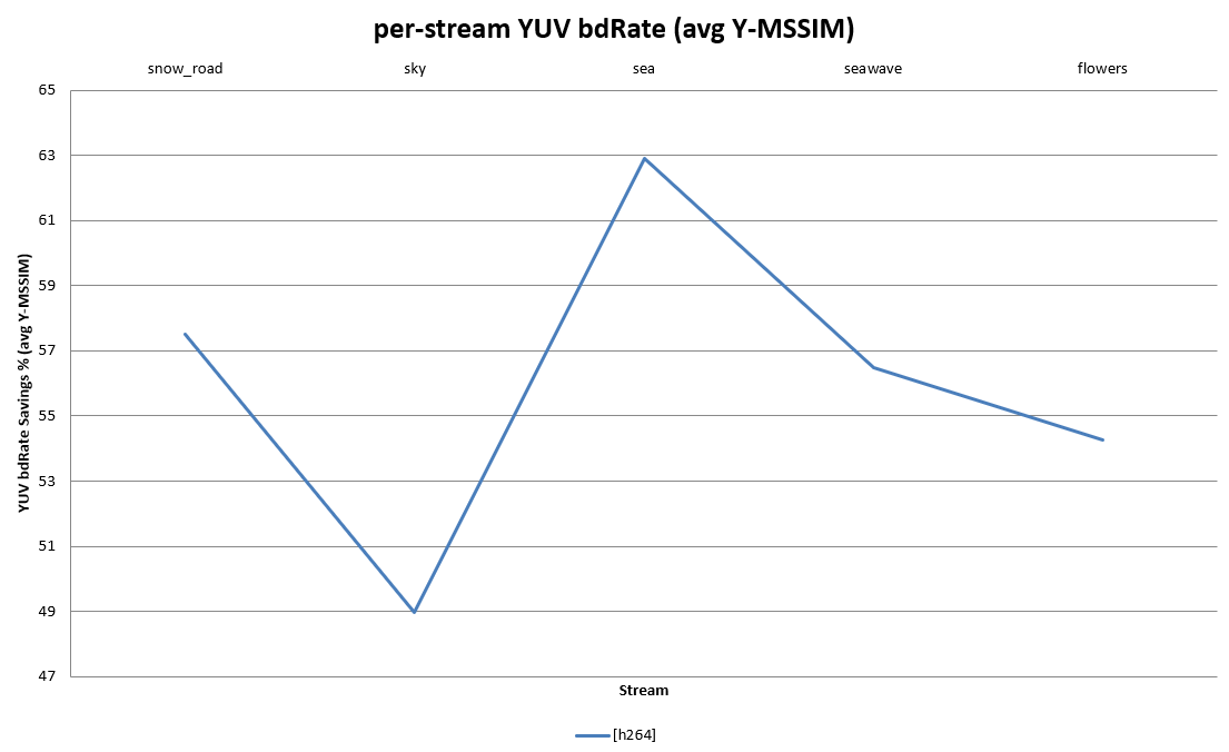
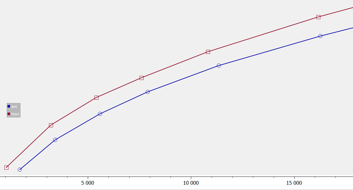
Then look at RD-curves.
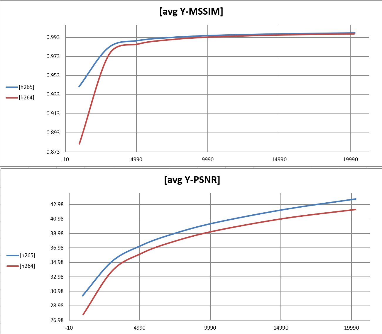
They demonstrate dependency bitrate from average metric value - Y-PSNR, Y-MSSIM. I would mark the higher plot of the better quality. On the sheet with RD-curves, we can see BD-rate info in percentage how codec in one case is better than the other one. Green color means h265 codec shows by 35.17% in avg Y-MSSIM metric and by 25.32% in avg Y-PSNR better quality than h264.
Performance
The next step is checking performance. We should know the average encoding speed for each bitrate in frames per second - FPS. Take the same command modes as for the encoding step in the quality part in the picture below.
tb::stages:
- model: q = 5, mode = frames
- label: encoding
instruction: encode()
tb::instructions:
- encode:
- label: encoding
- command: encode_tool {:args.codec}
- args:
- name: bitrate
call: '-b {:args.bitrate}' - name: input_stream
call: '-i {}'
value: '{:streams.stream_name}.yuv' - name: encoded_file
call: '-o {}
value: 'null'
- name: bitrate
Make encoding several times, in the example we run with param q=5 in the model section. It will run the same command more than one time and count the average value in FPS. We should point out to our tool that we want to get results in the FPS, make mode=frames. Also, we have the opportunity to get results in seconds - mode=sec.
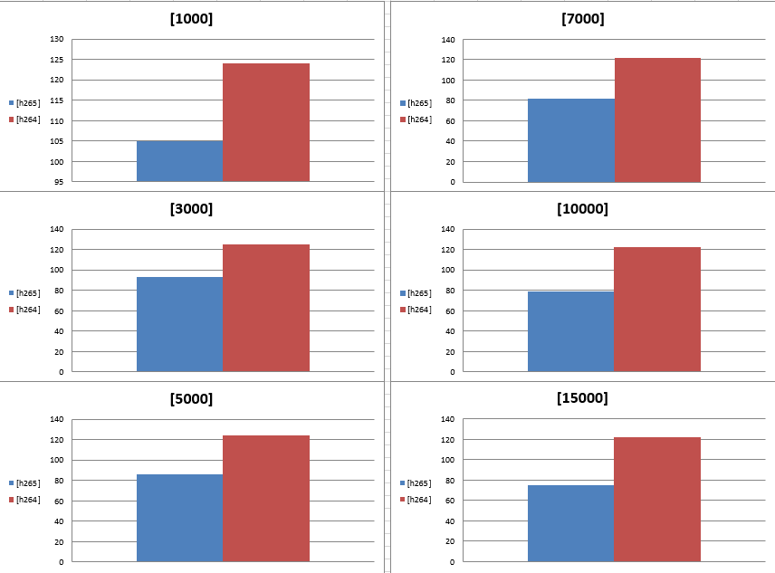
These diagrams show that encoding with one codec is faster than with another one.
Summary report
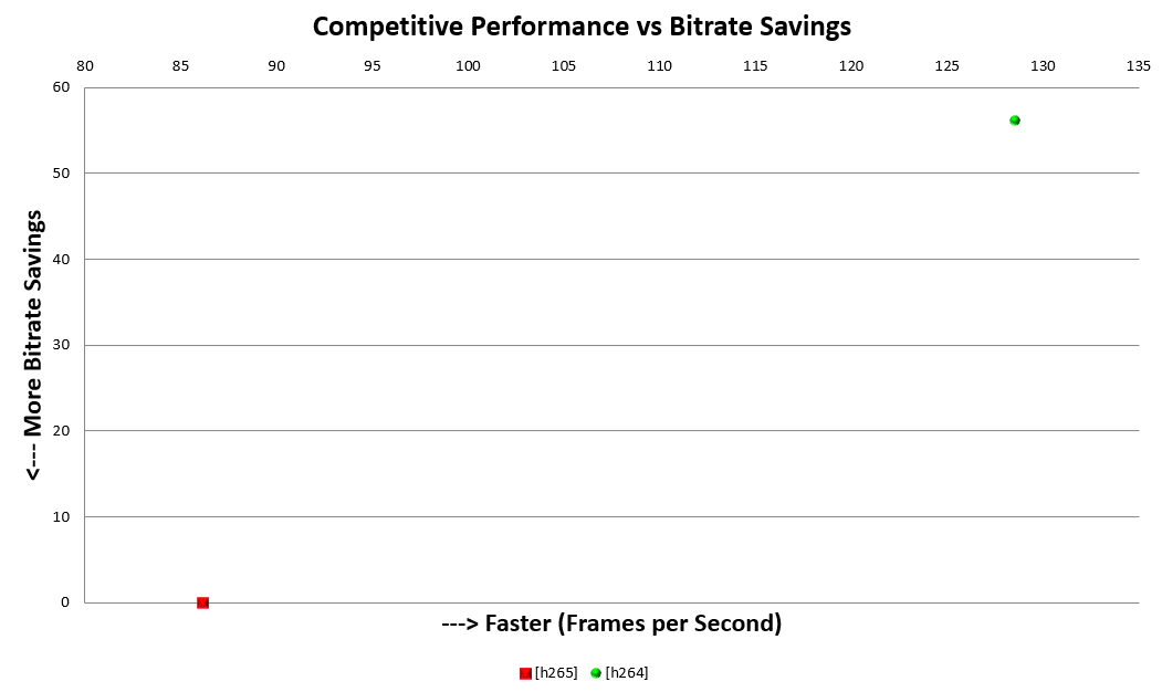
The latest part is the summary report pages. It will show the general picture of quality for all streams and dependency quality from performance. We took the h265 codec as a reference and built a dependency plot. It demonstrates the efficient encoding difference between codecs. If there are values below zero, it means that the quality is better.
The following graphic is the competitive performance versus bitrate saving. Axe directions point to bitrate saving and speed in FPS. It means that h264 is faster than h265 (we saw the same in performance diagrams), but h265 wins in bitrate saving.
Using VQProbe
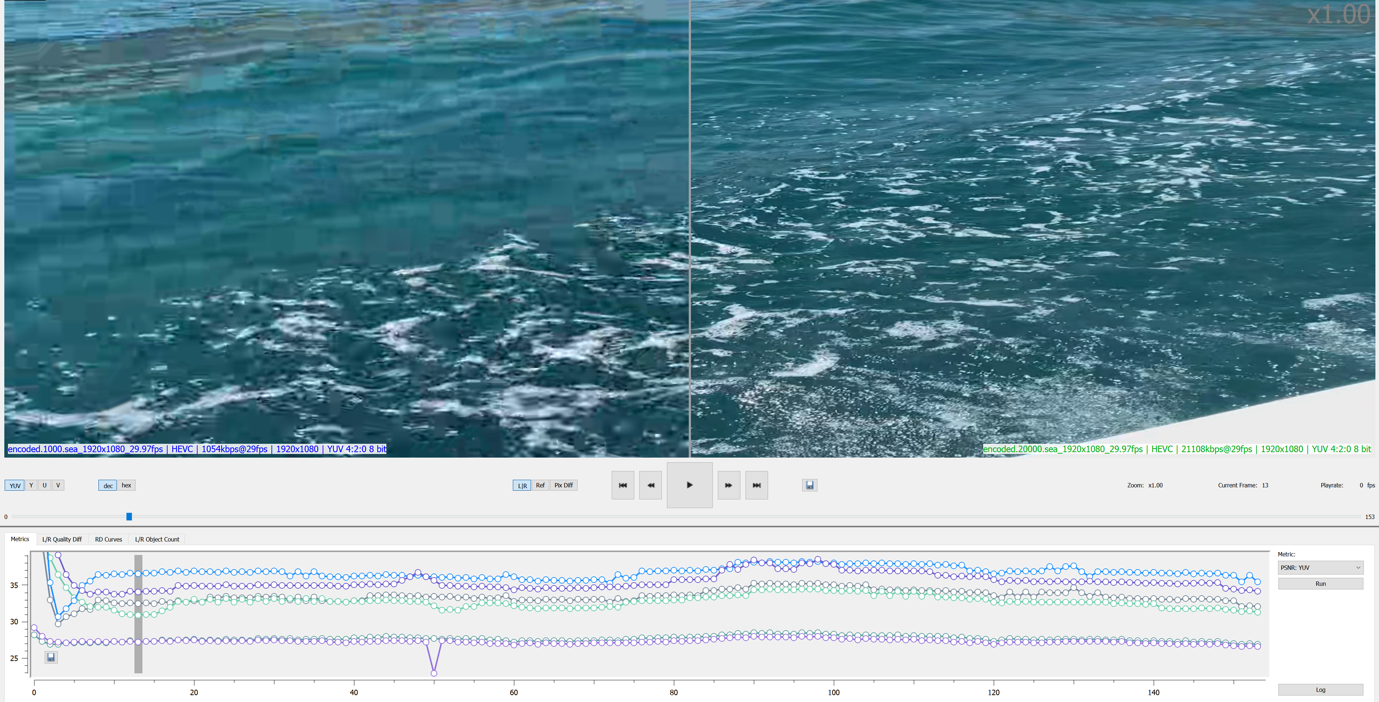
The central part shows the quality difference using our visual instrument VQProbe. This tool is helpful for subjective and objective comparison of video quality. In general, VQProbe’s interface looks like this:
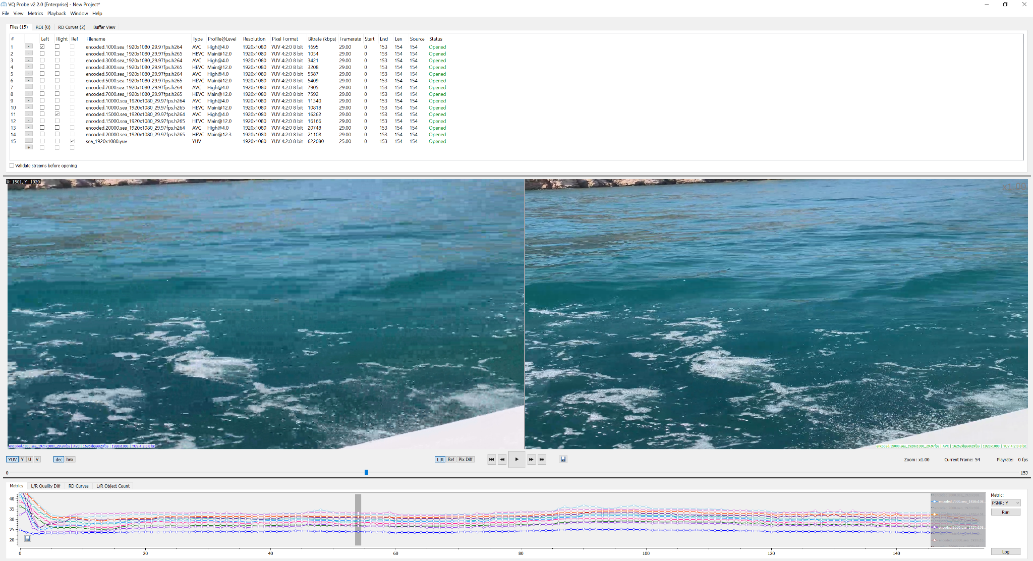
You can see frame difference or build per-frame metrics, RD-curves and compare the quality between streams. Let's choose, for example, two encoded streams with h264 codec and different bitrates, compare them.


Pay attention that on the top frame, the quality is worse (1000 Mbits) than on the bottom frame (15000 Mbits). This difference is caused by encoding the second stream with a bigger bitrate.
Build per-frame metrics for all streams.
So create RD-curves for each codec.
VQProbe has the capability to build per-frame metrics for all streams, look at video frames distinctions, research results, and find better options that we should use for quality video.